Replacing the Grid in the CP2K-generated UPF File

Problem

My repository gth2upf is found that it cannot reproduce the standard QE HGH-PBE UPF, giving different absolute energies and relative energies. While the HGH-PBE curve looks reasonable, the GTH-PBE curve is unphysical.

The two UPFs are generally agree, but the radial grid (rmax and RAB) are different. I guess this is the origin of the problem.

The First Investigation

Trace the related code in cpmd2upf and in CP2K ATOM module (atom_write_upf function), find:

cpmd2upf uses the fixed log grid (see the mesh formula below), where z is the atomic number (e.g. C: Z=6), dx(amesh) is fixed to 0.0125, and rmax is thus determined by the element type and the total number of grid points (mesh).

   IF ( .not. grid_read ) THEN
      xmin = -7.0d0
      amesh=0.0125d0
      rmax =100.0d0
      PRINT '("A radial grid must be provided. We use the following one:")'
      PRINT '("r_i = e^{xmin+(i-1)*dx}/Z, i=1,mesh, with parameters:")'
      PRINT '("Z=",f6.2,", xmin=",f6.2," dx=",f8.4," rmax=",f6.1)', &
            z, xmin, amesh, rmax
      mesh = 1 + (log(z*rmax)-xmin)/amesh
      mesh = (mesh/2)*2+1 ! mesh is odd (for historical reasons?)
      ALLOCATE (r(mesh))
      DO i=1, mesh
         r(i) = exp (xmin+(i-1)*amesh)/z
      ENDDO
      PRINT '(I4," grid points, rmax=",f8.4)', mesh, r(mesh)
      grid_read = .true.
   ENDIF

cp2k: According to the mesh part of atom_write_upf, PP_R is the value of atom%basis%grid%rad, and PP_RAB is the value of atom%basis%grid%wr(i)/atom%basis%grid%rad2(i).

       WRITE (iw, '(T4,A)') '<PP_MESH'
       WRITE (iw, '(T8,A)') 'dx="1.E+00"'
       CALL compose(string, "mesh", ival=nr)
       WRITE (iw, '(T8,A)') TRIM(string)
       WRITE (iw, '(T8,A)') 'xmin="1.E+00"'
       rmax = MAXVAL(atom%basis%grid%rad)
       CALL compose(string, "rmax", rval=rmax)
       WRITE (iw, '(T8,A)') TRIM(string)
       WRITE (iw, '(T8,A)') 'zmesh="1.E+00">'
       WRITE (iw, '(T8,A)') '<PP_R type="real"'
       CALL compose(string, "size", ival=nr)
       WRITE (iw, '(T12,A)') TRIM(string)
       WRITE (iw, '(T12,A)') 'columns="4">'
       IF (up) THEN
          WRITE (iw, '(T12,4ES25.12E3)') (atom%basis%grid%rad(i), i=1, nr)
       ELSE
          WRITE (iw, '(T12,4ES25.12E3)') (atom%basis%grid%rad(i), i=nr, 1, -1)
       END IF
       WRITE (iw, '(T8,A)') '</PP_R>'
       WRITE (iw, '(T8,A)') '<PP_RAB type="real"'
       CALL compose(string, "size", ival=nr)
       WRITE (iw, '(T12,A)') TRIM(string)
       WRITE (iw, '(T12,A)') 'columns="4">'
       IF (up) THEN
          WRITE (iw, '(T12,4ES25.12E3)') (atom%basis%grid%wr(i)/atom%basis%grid%rad2(i), i=1, nr)
       ELSE
          WRITE (iw, '(T12,4ES25.12E3)') (atom%basis%grid%wr(i)/atom%basis%grid%rad2(i), i=nr, 1, -1)
       END IF
       WRITE (iw, '(T8,A)') '</PP_RAB>'
       WRITE (iw, '(T4,A)') '</PP_MESH>'

Continue to search where ‘rad’ and ‘wr’ are assigned: (the ‘r’ in the code block below is assigned to ‘rad’)

 ! qs_grid_atom.F, #596
 ! r will be assigned to rad
 SELECT CASE (radial_quadrature)

 CASE (do_gapw_gcs)
    ! Gauss-Chebyshev quadrature formula of the second kind
    ! u [-1,+1] -> r [0,infinity] =>  r = (1 + u)/(1 - u)
    DO i = 1, n
       t = REAL(i, dp)*f
       x = COS(t)
       w = f*SIN(t)**2
       r(i) = (1.0_dp + x)/(1.0_dp - x)
       r2(i) = r(i)**2
       wr(i) = w/SQRT(1.0_dp - x**2)
       wr(i) = 2.0_dp*wr(i)*r2(i)/(1.0_dp - x)**2
    END DO

 CASE (do_gapw_gct)
    ! Transformed Gauss-Chebyshev quadrature formula of the second kind
    DO i = 1, n
       t = REAL(i, dp)*f
       cost = COS(t)
       sint = SIN(t)
       sint2 = sint**2
       x = REAL(2*i - n - 1, dp)/REAL(n + 1, dp) - &
          2.0_dp*(1.0_dp + 2.0_dp*sint2/3.0_dp)*cost*sint/pi
       w = 16.0_dp*sint2**2/REAL(3*(n + 1), dp)
       r(n + 1 - i) = (1.0_dp + x)/(1.0_dp - x)
       r2(n + 1 - i) = r(n + 1 - i)**2
       wr(n + 1 - i) = 2.0_dp*w*r2(n + 1 - i)/(1.0_dp - x)**2
    END DO

 CASE (do_gapw_log)
    ! Transformed Gauss-Chebyshev quadrature formula of the second kind
    ! u [-1,+1] -> r [0,infinity] => r = ln(2/(1 - u))/ln(2)
    DO i = 1, n
       t = REAL(i, dp)*f
       cost = COS(t)
       sint = SIN(t)
       sint2 = sint**2
       x = REAL(2*i - n - 1, dp)/REAL(n + 1, dp) - &
          2.0_dp*(1.0_dp + 2.0_dp*sint2/3.0_dp)*cost*sint/pi
       w = 16.0_dp*sint2**2/REAL(3*(n + 1), dp)
       r(n + 1 - i) = LOG(2.0_dp/(1.0_dp - x))/LOG(2.0_dp)
       r2(n + 1 - i) = r(n + 1 - i)**2
       wr(n + 1 - i) = w*r2(n + 1 - i)/(LOG(2.0_dp)*(1.0_dp - x))
    END DO

From CP2K’s code we can see it supports three types of radial grid: do_gapw_gcs, do_gapw_gct and do_gapw_log.

Trace the variable radial_quadrature can we find the corresponding parameter QUADRATURE:

QUADRATURE: enum= GC_LOG

Usage: QUADRATURE (GC_SIMPLE GC_TRANSFORMED GC_LOG)

Valid values:

GC_SIMPLE Gauss-Chebyshev quadrature

GC_TRANSFORMED Transformed Gauss-Chebyshev quadrature

GC_LOG Logarithmic transformed Gauss-Chebyshev quadrature

Algorithm to construct the atomic radial grids

Plot the grid data of the CP2K-generated upf file with each of the above three quadrature types, we find that none of them can reproduce the default grid used by cpmd2upf:

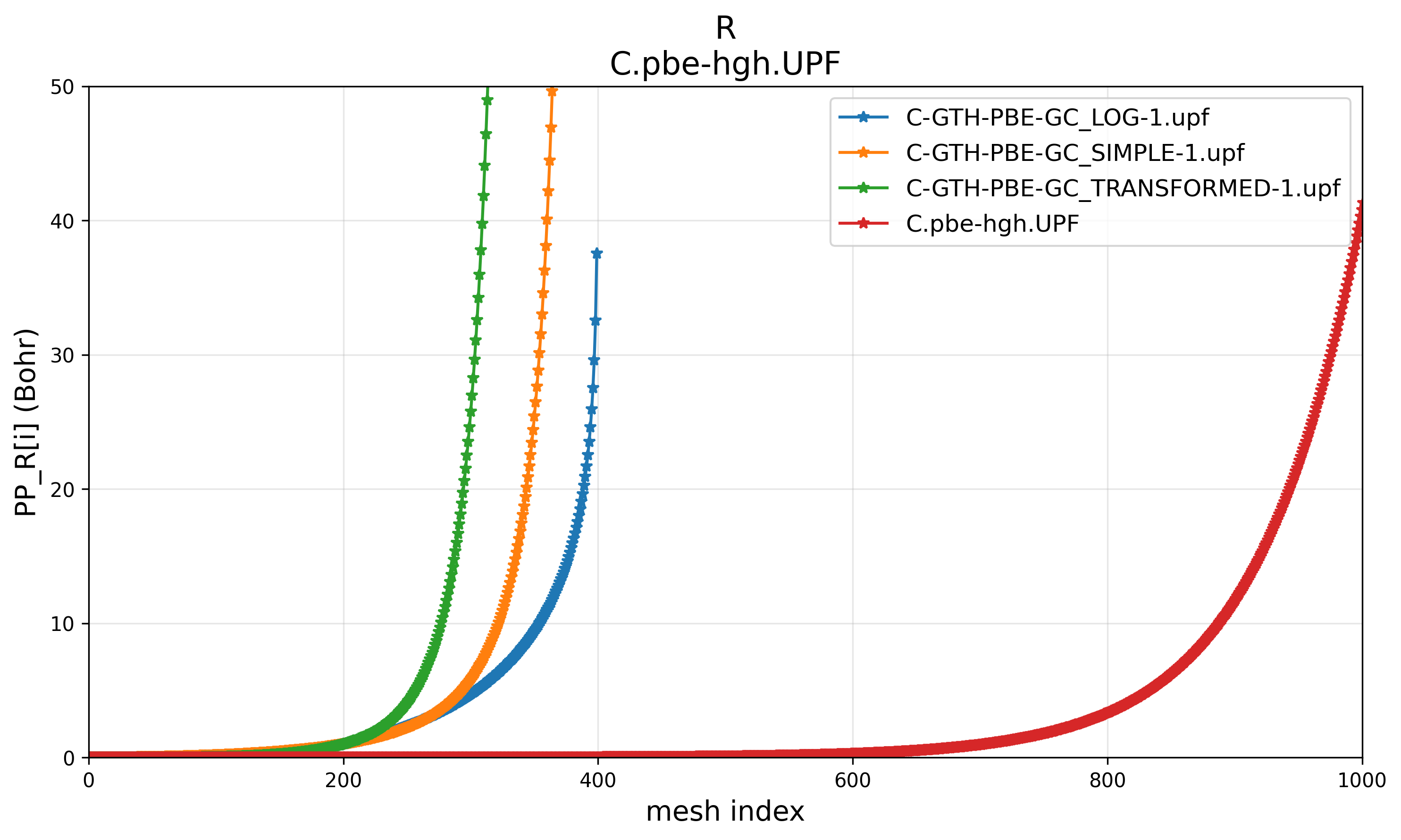
PP_R

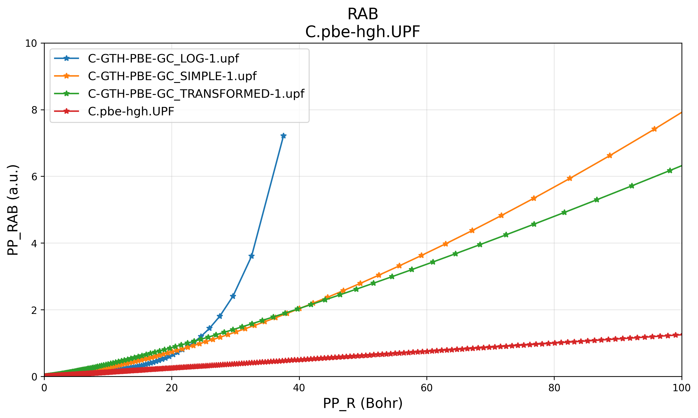
PP_RAB

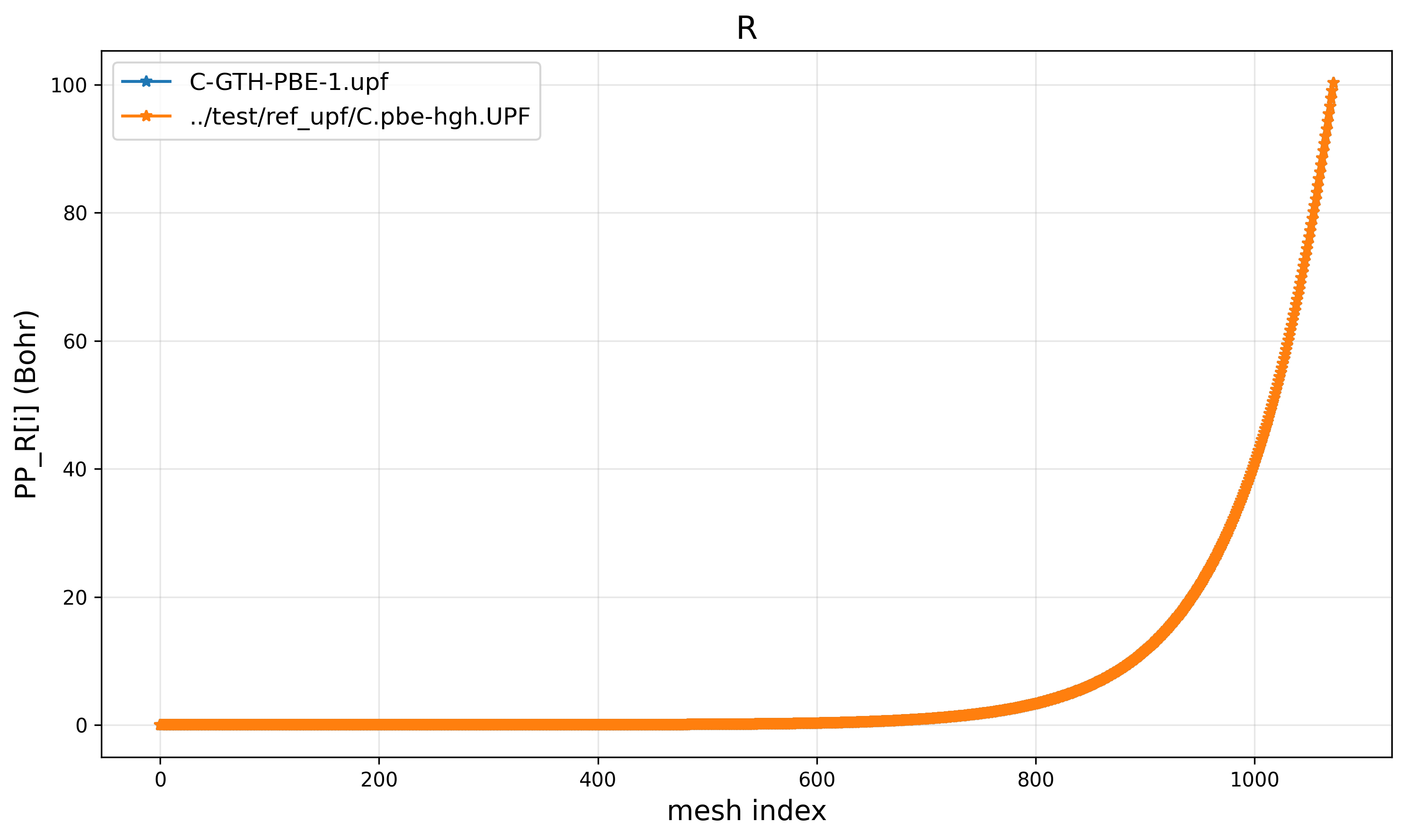
Another tunable parameter is GRID_POINTS, which controls the total number of radial grid points. The default value is 400. Unfortunately, changing this cannot control the curvature shape of PP_R and PP_RAB, and cannot even control the cutoff radius (rmax) exactly:

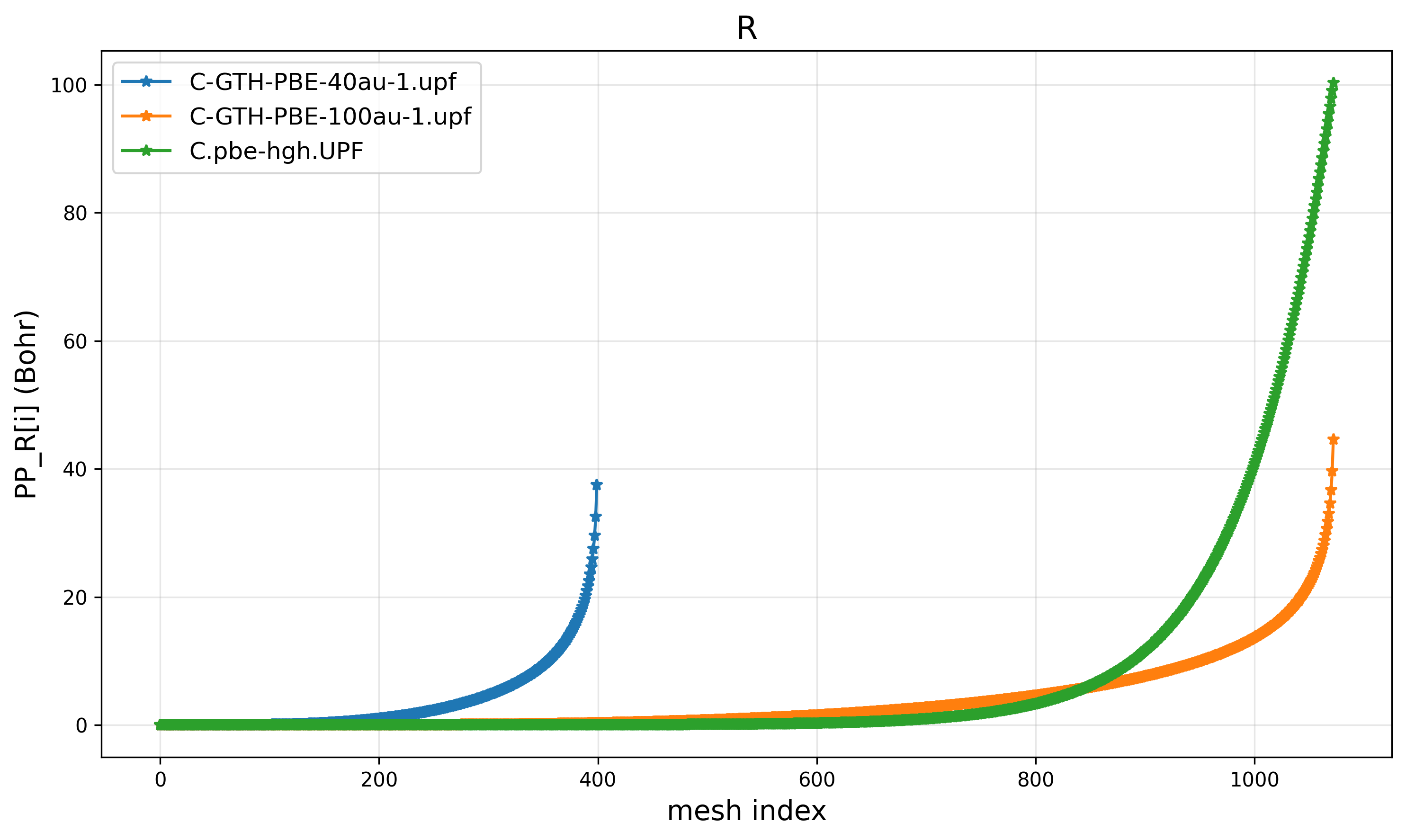
R vs. mesh index

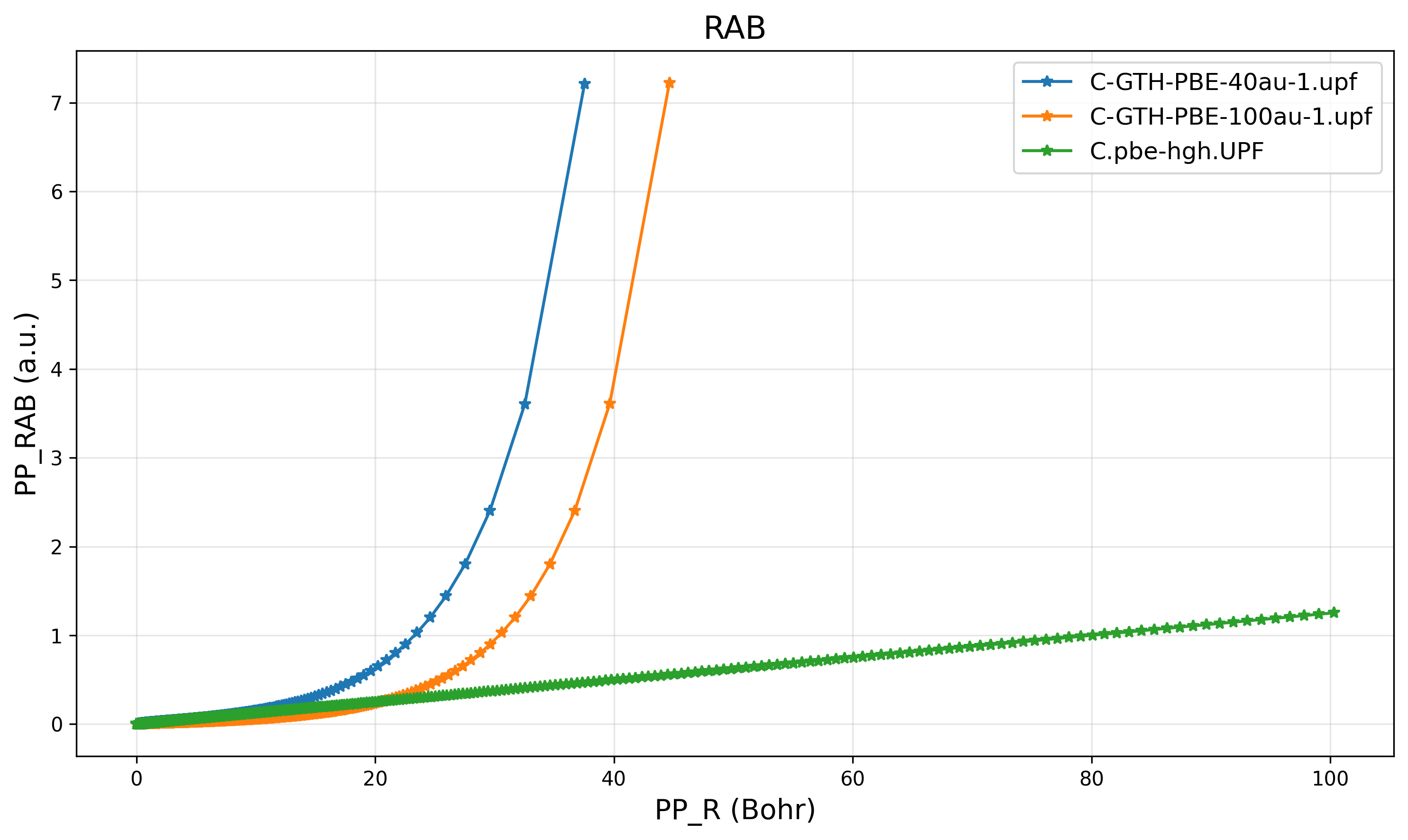
RAB vs. R

Thus, I must write a script by myself, to convert GTH format to UPF with the logarithmic radial grid of the formula in cpmd2upf by default.

Math Fitting

Using logarithmic y coordinate (plot.semilogy) to plot the grid step length dR, the result shows that C.pbe-hgh.UPF is log-gridded, while C-GTH-PBE-1.upf generated by cp2k is not.

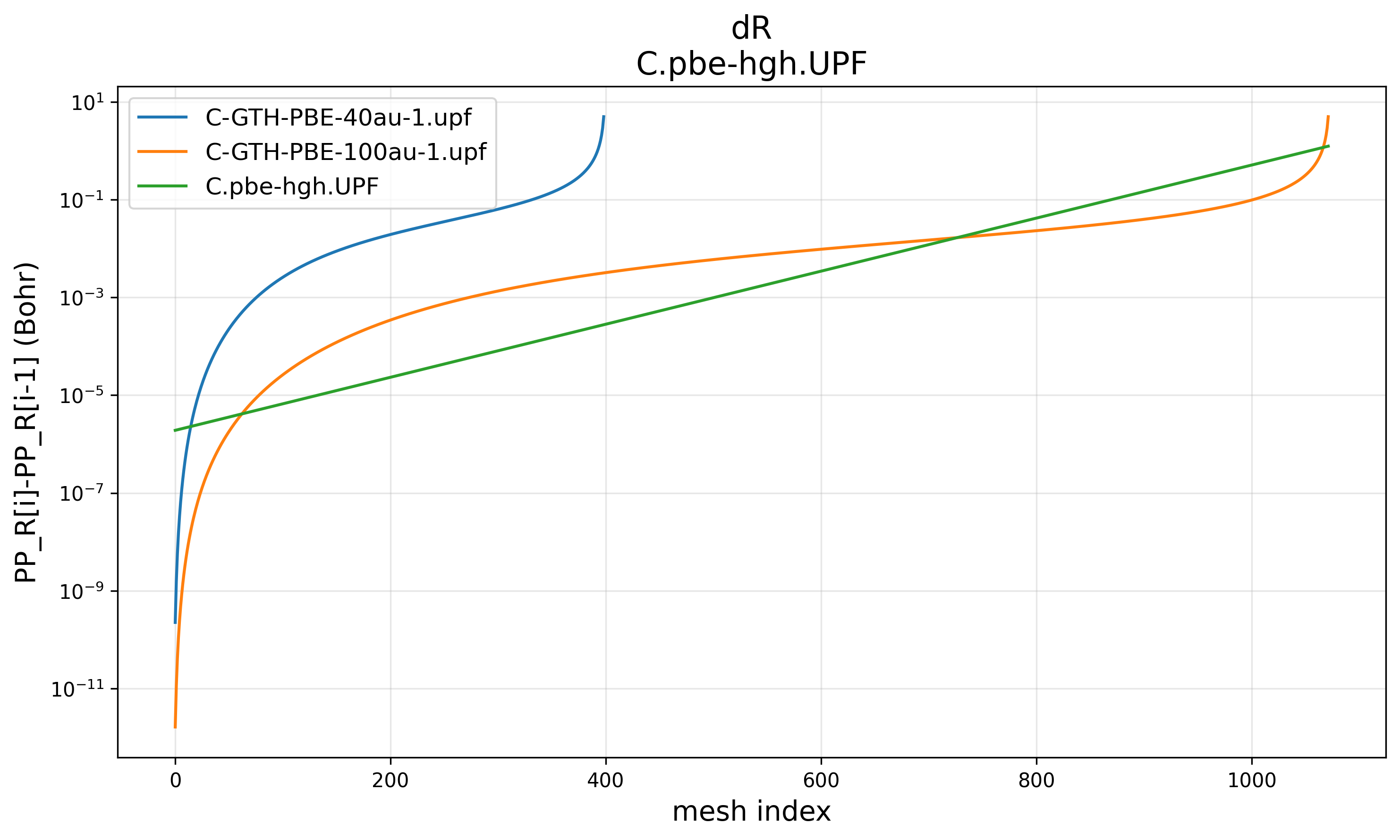
dR[i]=PP_R[i+1]-PP_R[i]

AI-agent based IDE Trae reminds me that the grid type in cp2k may be sinh, and helped me to write the fitting script. The result is amazing:

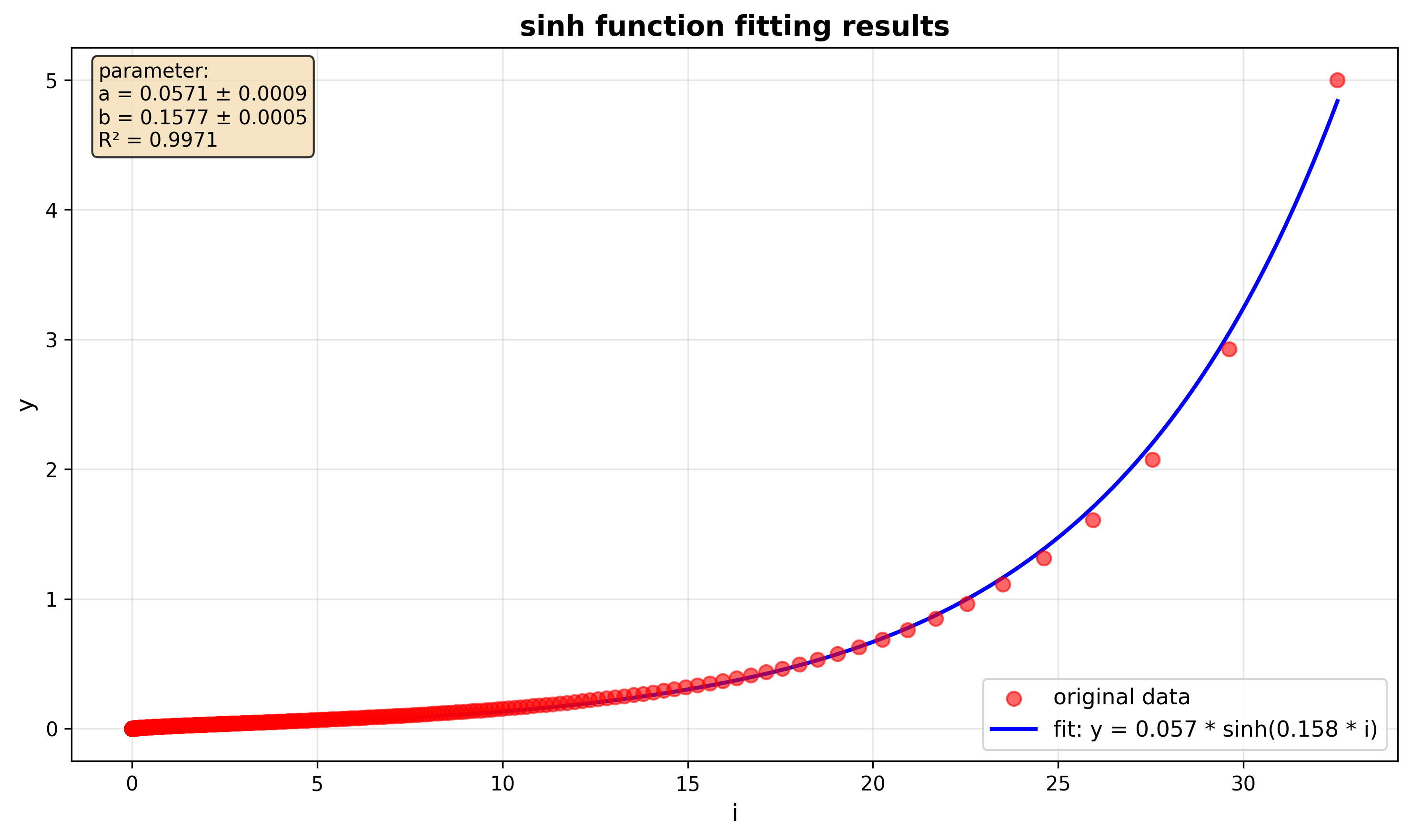
sinh fitting of dR generated by CP2K

After diving into the code, extract the two types of formulas (from GC_LOG in CP2K and from cpmd2upf respectively), plot and compare: \(\begin{aligned} r_{\text{cp2k}} & = \ln(2/(1 - x))/\ln(2) \\ r_{\text{cpmd2upf}} & = \exp(x)/z \end{aligned}\)

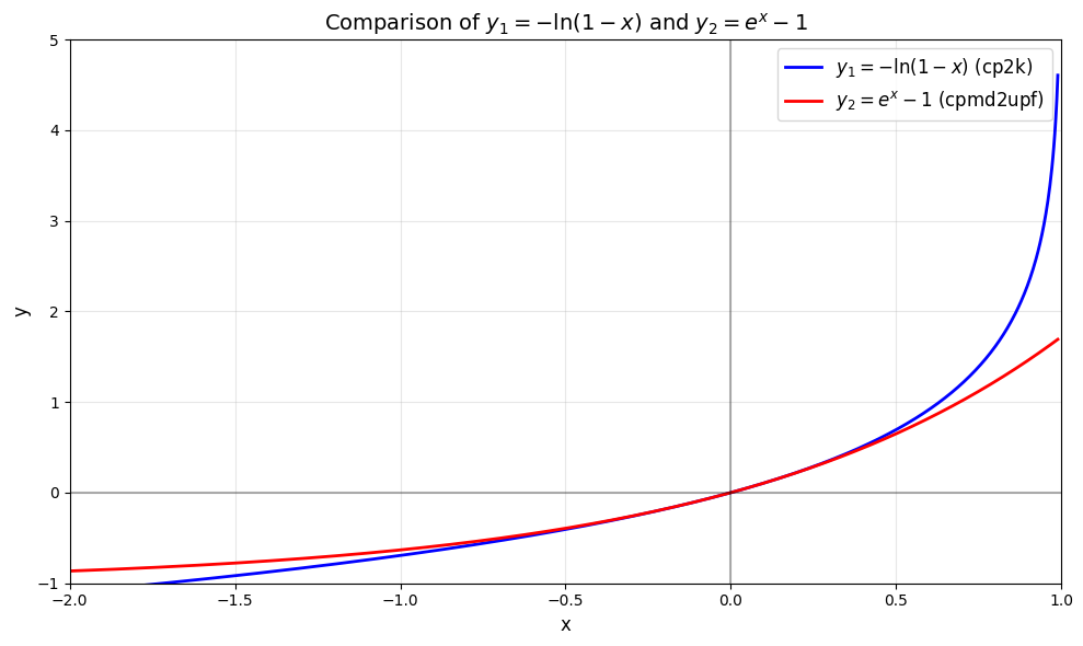
Compare -ln(1-x) and exp(x)-1

In [0, 1], compared to \(\exp(x)-1\), \(-\ln(1-x)\) increases more rapidly as \(x\) approaches 1, which makes the CP2K’s grid “denser near the neucleus, coarser outside”. I guess this is a special design for all-electron calculation.

Implementing the Quadrature Type “CPMD2UPF_DEFAULT”

Workflow (gth2upf.py):

Parse the input json file
Generate CP2K input file
Run CP2K
Parse the output upf file
Replace the grid
Interpolate the data (PP_LOCAL, PP_RHOATOM, PP_CHI, etc.)
Rewrite the upf file

Step 4-7 are implemented in upf_data.py.

Results show that the grid is the same as the reference file C.pbe-hgh.UPF, while the data matches the CP2K-generated C-GTH-PBE-1.upf.

PP_R

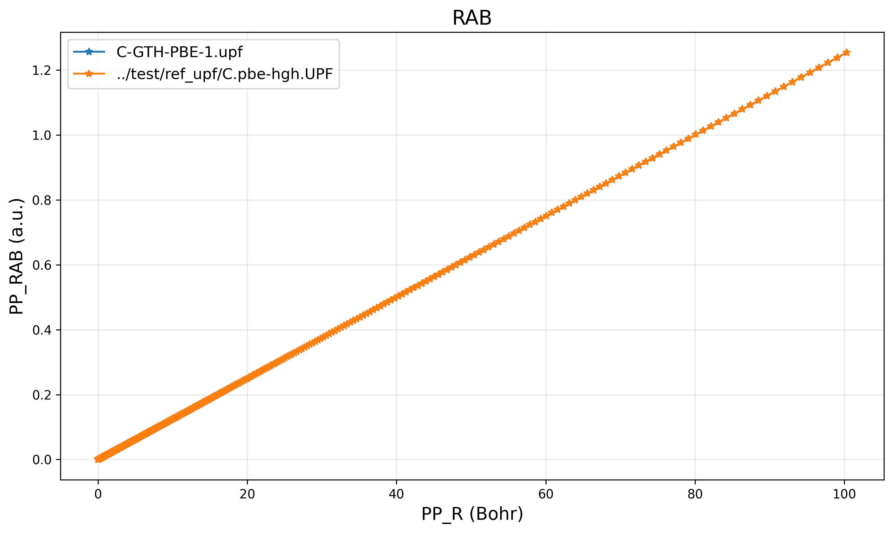
PP_RAB

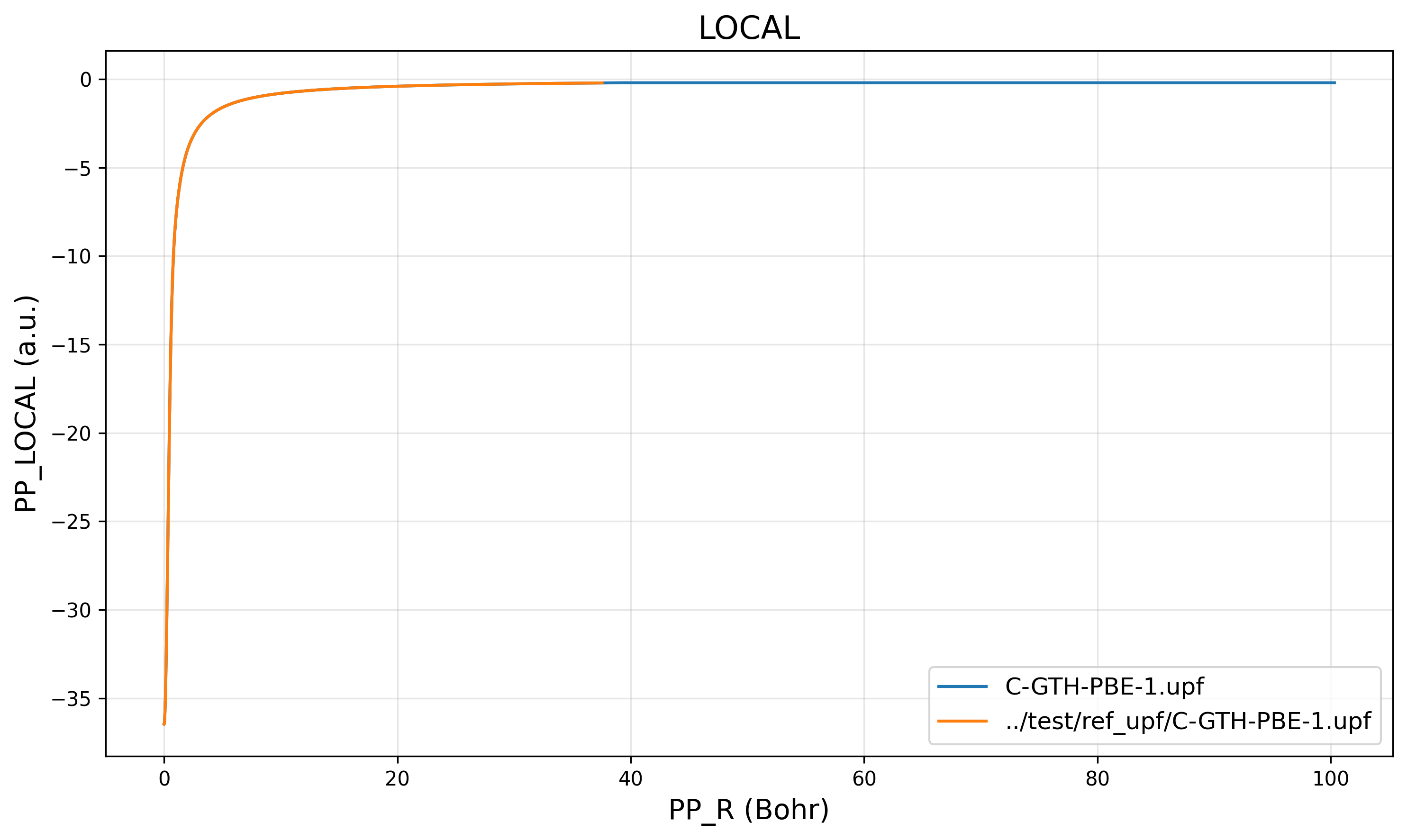
PP_LOCAL

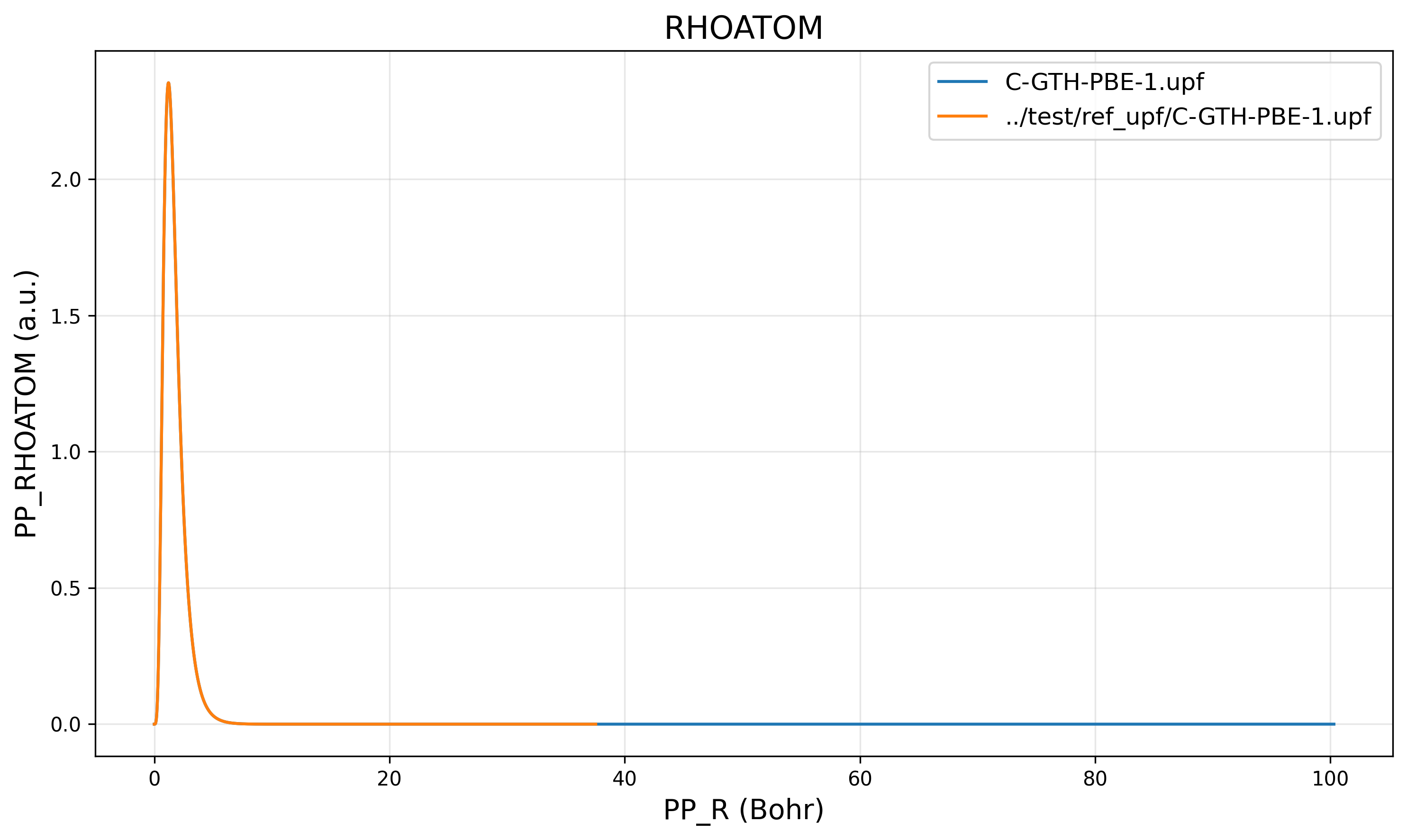
PP_RHOATOM

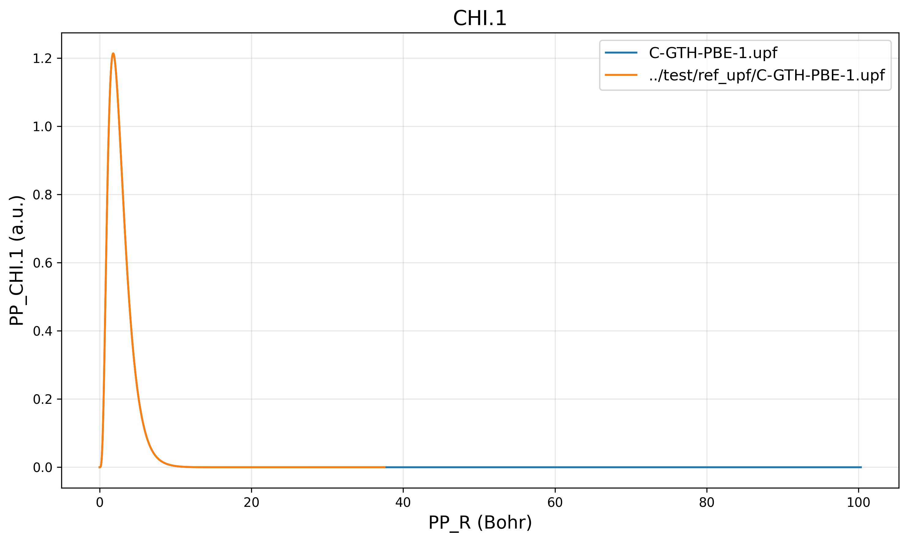
PP_CHI.1

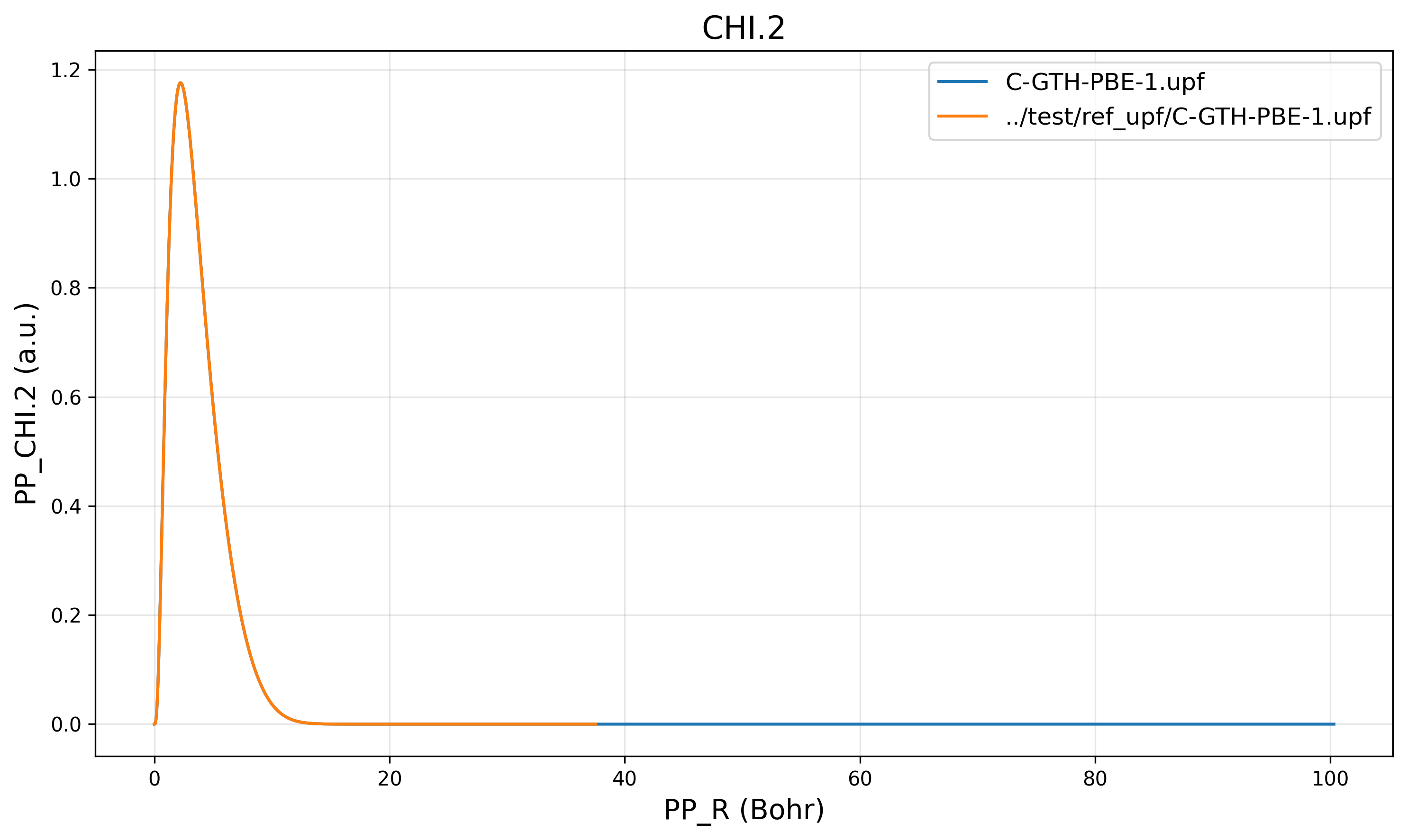
PP_CHI.2

Two steps to convert markdown file into pdf with GitHub Style

grip report.md --export tmp.html --user <username>
wkhtmltopdf --enable-local-file-access tmp.html report.pdf

If you want to remove the markdown filename on the left-upper conner of the pdf, comment out the header block including the filename in tmp.html between the two steps.

Problem

The First Investigation

Math Fitting

Implementing the Quadrature Type “CPMD2UPF_DEFAULT”

Two steps to convert markdown file into pdf with GitHub Style

Comments